Total scattering - Debye approach

Neutron or X-ray scattering static structure factor S(q) is defined as:

$${\frac{{1}}{{N}}} \sum_{{j,k}}^{} \left<\vphantom{ e^{\displaystyle{iq[{\bf {r}}_j-{\bf {r}}_k]}} }\right. \bf {r}_{j} \bf {r}_{k} \left.\vphantom{ e^{\displaystyle{iq[{\bf {r}}_j-{\bf {r}}_k]}} }\right>$$ (5.6)

where b_j et $\bf {r}_{j}^{}$ represent respectively the neutron or X-ray scattering length, and the position of the atom j. N is the total number of atoms in the system studied.
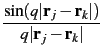
To take into account the inherent/volume averaging of scattering experiments it is necessary to sum all possible orientations of the wave vector q compared to the vector $\bf {r}_{j}^{}$ - $\bf {r}_{k}^{}$. This average on the orientations of the q vector leads to the famous Debye's equation:

$${\frac{{1}}{{N}}} \sum_{{j,k}}^{} {\frac{{\sin (q\vert{\bf {r}}_j-{\bf {r}}_k\vert)}}{{q\vert{\bf {r}}_j-{\bf {r}}_k\vert}}}$$ (5.7)

Nevertheless the instantaneous individual atomic contributions introduced by this equation [Eq. 5.7] are not easy to interpret. It is more interesting to express these contributions using the formalism of radial distribution functions [Sec. 5.2].
In order to achieve this goal it is first necessary to split the self-atomic contribution (j = k), from the contribution between distinct atoms:

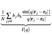$$\sum_{{j}}^{} \underbrace{{\frac{1}{N} \sum_{j\ne k} b_j b_k \frac{\sin (q\ver... ...r}}_k\vert)}{q\vert{\bf {r}}_j-{\bf {r}}_k\vert}}}_{{\displaystyle{I(q)}}}^{}$$ (5.8)

with c_j = $${\frac{{N_j}}{{N}}}$$.
    4π $$\sum_{{j}}^{}$$ c_jb_j²     represents the total scattering cross section of the material.
The function I(q) which describes the interaction between distinct atoms is related to the radial distribution functions through a Fourier transformation:

$$\int_{{0}}^{{\infty}} {\frac{{\sin qr}}{{qr}}}$$ (5.9)

where the function G(r) is defined using the partial radial distribution functions [Eq. 5.4]:

$$\sum_{{\alpha,\beta}}^{}$$ (5.10)

where c_α = $${\frac{{N_\alpha}}{{N}}}$$ and b_α represents the neutron or X-ray scattering length of species α.
G(r) approaches - - $$\sum_{{\alpha,\beta}}^{}$$ c_αb_α c_βb_β for r = 0, and 0 for r→∞.
Usually the self-contributions are substracted from equation [Eq. 5.8] and the structure factor is normalized using the relation:

$${\frac{{I(q)}}{{\displaystyle{\langle b^{2} \rangle}}}} \left(\vphantom{\sum_{\alpha} c_{\alpha} b_{\alpha} }\right. \sum_{{\alpha}}^{} \left.\vphantom{\sum_{\alpha} c_{\alpha} b_{\alpha} }\right)^{{2}}_{}$$ (5.11)

It is therefore possible to write the structure factor [Eq. 5.7] in a more standard way:

$$\int_{{0}}^{{\infty}} {\frac{{\sin qr}}{{qr}}} \bf {g}$$ (5.12)

where $\bf {g}$(r) (the radial distribution function) is defined as:

$$\bf {g} {\frac{{\displaystyle{\sum_{\alpha,\beta}} c_{\alpha} b_{\alpha}... ...beta} b_{\beta} g_{\alpha\beta}(r) }}{{\displaystyle{\langle b^{2} \rangle}}}}$$ (5.13)

In the case of a single atomic species system the normalization allows to obtain values of S(q) and $\bf {g}$(r) which are independent of the scattering factor/length and therefore independent of the measurement technique. In most cases, however, the total S(q) and $\bf {g}$(r) are combinations of the partial functions weighted using the scattering factor and therefore depend on the measurement technique (Neutron, X-rays ...) used or simulated.

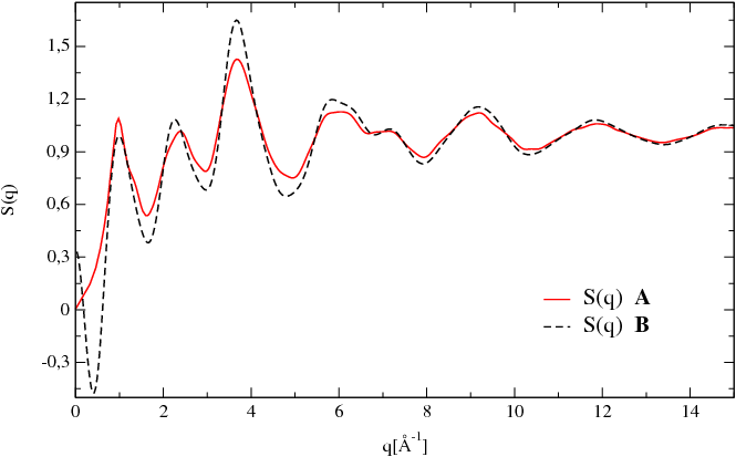
Figure 5.4: Total neutron structure factor for glassy GeS₂ at 300 K - A Evaluation using the atomic correlations [Eq. 5.7], B Evaluation using the pair correlation functions [Eq. 5.12].

Figure [Fig. 5.4] presents a comparison bewteen the calculations of the total neutron structure factor done using the Debye relation [Eq. 5.7] and the pair correlation functions [Eq. 5.12]. The material studied is a sample of glassy GeS₂ at 300 K obtained using ab-initio molecular dynamics. In several cases the structure factor S(q) and the radial distribution function $\bf {g}$(r) [Eq. 5.13] can be compared to experimental data. 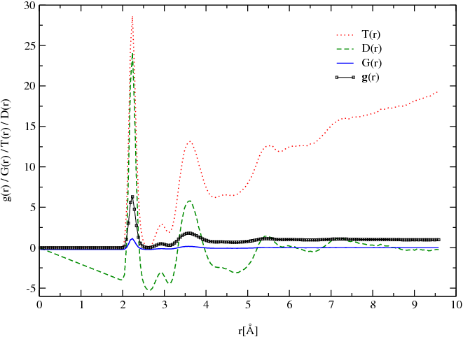To simplify the comparison I.S.A.A.C.S. computes several radial distribution funcrions used in practice suh as G(r) defined [Eq. 5.10], the differential correlation function D(r), $\bf {G}$(r), and the total correlation function T(r) defined by:

D(r)  =  4πrρ G(r) (5.14)

$$\bf {G} {\frac{{D(r)}}{{\langle b^{2} \rangle}}}$$ T(r)  =  D(r)  +  4πrρ 〈b²〉

$\bf {g}$(r) equals zero for r = 0 and approaches 1 for r→∞.
D(r) equals zero for r = 0 and approaches 0 for r→∞.
$\bf {G}$(r) equals zero for r = 0 and approaches 0 for r→∞.
T(r) equals zero for r = 0 and approaches ∞ for r→∞.
This set of functions for a model of GeS₂ glass (at 300 K) obtained using ab-intio molecular dynamics is presented in figure [Fig. 5.5].

Figure 5.5: Exemple of various distribution functions neutron-weighted in glassy GeS₂ at 300 K.

I.S.A.A.C.S. can compute, for the case of x-ray or neutrons, the following functions:

•

S(q) and Q(q)  =  q[S(q) - 1.0] [9,10] computed using the Debye equation

•

S(q) and Q(q)  =  q[S(q) - 1.0] [9,10] computed using the Fourier transform of the $\bf {g}$(r)

•

$\bf {g}$(r) and $\bf {G}$(r) computed using the standard real space calculation

•

$\bf {g}$(r) and $\bf {G}$(r) computed using the Fourier transform of the structure factor calculated using the Debye equation