SPSS On-Line Training Workshop

SPSS On-Line Training Workshop |
|
|
 In this Tutorial: |
|
In this on-line workshop, you will find many movie clips. Each movie clip will demonstrate some specific usage of SPSS.
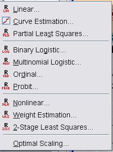
Linear regression: Regression modeling is a technique for modeling a response variable, which is often assumed to follow a normal distribution, using a set of independent variables. The least square method is usually applied for estimating the regression parameters. Variable selection and model diagnostics are important tasks for building regression models.
|
Method: This lets you select how independent variables are entered into the analysis. The "Enter" method enters all variables at the same time. The other methods involve some sort of step-wise regression. |
The linear regression dialog box has the following sub-menus:
Statistics: Many statistics including regression coefficient estimates, goodness-of-fit statistics and partial correlations can be requested. By default Estimates and Model fit are selected. R-squared change is needed for variable selection methods. If you want to check for collinearity problems, you can select “Collinearity diagnostics”. You can make other selections, if needed. | |
Plots: You have the option of plotting the residuals, obtaining the histogram or the normal probability plot of the standardized residuals. | |
Save: You can save some of the results of the analysis, either to the data editor or to a new file. | |
Options: If you are doing stepwise regression, you can change the criteria for entry and removal under this submenu. You can select how missing values should be treated |
The following two movie clips are developed for regression modeling.
![]() Click
here to watch Linear Regression
Click
here to watch Linear Regression
![]() Click
here to watch Stepwise Regression
Click
here to watch Stepwise Regression
The data set for demonstrating regression modeling is the Body Fat data set. See Data Set page for details. The dependent variable is the amount of body fat, and the independent variables are triceps skinfold thickness, thigh circumference, and mid-arm circumference.
Binary Logistic Regression: This is used to determine factors that affect the presence or absence of a characteristic when the dependent variable has two levels. In the dialog box, you select one dependent variable and your independent variables, which may be factors or covariates.
|
Method- This lets you select how independent variables are entered into the analysis. The "Enter" method enters all variables at the same time. The other methods involve some sort of step-wise regression. | |
|
Selection Variable: This is used if you want to limit your analysis to certain levels of a variable. |
The following is the sub-menu on the main dialog box:
Categorical: Here is where you identify categorical variables and specify how you want this data compared. | |
Save: This allow you to save output as new variables in the data editor window. | |
Options: If you are doing stepwise regression, this is where you can set your entry and removal criteria. Another option that can be checked here is the "CI for exp(B):". This gives you the odds ratio and is helpful in interpretation of parameter estimates. |
Multinomial Logistic Regression: This is used to determine factors that affect the presence or absence of a characteristic when the dependent variable has three or more levels. In the dialog box, you select one dependent variable and your independent variables, which may be factors or covariates. The dialog box has the following submenus:
Model: By default, a main effect model is fitted. In this submenu, you can specify a custom model or a variable selection method. | |
|
Statistics: In this submenu, you can request for many statistics including goodness-of-fit statistics for the model. | |
Criteria: This allows you to specify the criteria for the iterations during model estimation. | |
Categorical: Here is where you identify categorical variables and specify how you want this data compared. | |
|
Options: This allows you to specify options for the stepwise method. You can also specify the Deviance or Pearson as the dispersion scaling value. This is used to correct the estimate of the parameter covariance matrix. | |
|
Save: This allow you to save some variables to the working data file or to an external data file. |
![]() Click
here to watch Logistic Regression
Click
here to watch Logistic Regression
Ordinal Regression: This is used to fit an ordinal dependent (response) variable on a number of predictors (which can be factors or covariates). In general, the ordinal variable has more than two levels. For example, a variable that can take the values low, medium or high.
Nonlinear Regression:
This estimates a nonlinear model
relating one dependent variable to a number of independent variables. Note that
![]() , is still a linear regression model since
, is still a linear regression model since ![]() can be defined as
can be defined as
![]() to obtain a linear
regression model
to obtain a linear
regression model
![]() . To use the nonlinear procedure, you need to know the form of
the nonlinear relationship. In the “Nonlinear Regression” dialog box, specify
the dependent variable and the model expression for the nonlinear relationship.
Movie Clip is not available , See SPSS help for details
. To use the nonlinear procedure, you need to know the form of
the nonlinear relationship. In the “Nonlinear Regression” dialog box, specify
the dependent variable and the model expression for the nonlinear relationship.
Movie Clip is not available , See SPSS help for details
The data set for demonstrating the logistic regression is the Disease data set. See the Data Set page for details. The dependent variable, Disease is a binary variable with the presence of the disease represented by a 1 or absence of the disease which is represented by a 0. The covariates we will be using will be age, which is a quantitative variable, social class, which is a categorical variable with 3 levels (upper, lower, and middle), sector, which is categorical and represents two sectors within the city, and account, which is also categorical (those with savings accounts and those without).
![]()
![]()
This online SPSS Training Workshop is developed by Dr Carl Lee, Dr Felix Famoye , student assistants Barbara Shelden and Albert Brown , Department of Mathematics, Central Michigan University. All rights reserved.